import pandas as pd
import numpy as np
import matplotlib.pyplot as plt
import seaborn as sns

A/B test

두 개의 그룹을 비교하여 차이가 있는지 판단
A/B test, T-test… 등으로 불림

임의화(randomnization)

공정해야 한다라는 것의 의미는?
- 실험에서 고려한 의도적인 차이에 의한 효과(처리효과,treatment 효과)외에
- 다른 요인의 차이에 의해 두 그룹간에 효과의 차이가 나타날 가능성이 있으면 안된다는 것.
- ex) 신약의 효과를 입증하고자 하는 실험. 신약과 기존약의 차이외에 다른 요인이 없어야함.(인종,성별,나이,…)
두 그룹간의 비교가 공정하지 못하다면?
- 효과가 차이가 날 경우 진짜 의도한 차이에 의한 효과가 아니기에 과대평가 할 수 있음.
- 효과가 차이가 안날 수도 있는데 이 경우 과소평가.
- 두 경우 모두, 실험에서 고려한 의도적인 차이가 결과에 미치는 영향을 정확히 파악할 수 없음.
목적 : 두 그룹에 대한 비교는 반드시 공정해야 함. 이때 공정함을 구현하는 방법.
어떻게 구현?
- 두 개의 처리 중 하나를 실험대상에게 지정(배정)할때
- 처리의 배정을 임의로 결정(randomly assigned treatment) 하자.
  - 평균적으로 처리 외의 다른 요인들이 두 그룹에서 유사하게 나타나게 할 수 있음.
  - 두 그룹이 유사하기 때문에 처리외의 다른 요인으로 인한 효과의 차이가 나타날 가능성이 적음.

임의화 실험의 예시

임의화 구현

1874명의 사람들을 임상실험에 참가하는 환자들이라 가정하고 임의화 실험을 해보자

url = "https://ilovedata.github.io/teaching/bigdata2/data/physical_test_2018_data.csv"
physical_data = pd.read_csv(url)
twogroup = physical_data[["TEST_AGE","TEST_SEX","ITEM_F001","ITEM_F002"]].rename(columns = {"ITEM_F001":"height","ITEM_F002":"weight"})
twogroup

	TEST_AGE	TEST_SEX	height	weight
0	33	M	159.2	57.2
1	48	F	155.8	52.9
2	22	M	175.2	96.2
3	29	M	178.7	79.4
4	31	F	160.1	50.2
...	...	...	...	...
1869	18	M	179.8	79.8
1870	29	F	156.3	51.4
1871	19	M	173.9	64.5
1872	66	F	141.3	54.9
1873	51	F	155.5	59.9

1874 rows × 4 columns

각 환자에게 A,B 중 어떤 약을 투약할지 임의로 지정!

N,p = twogroup.shape
treatment = np.repeat("A",N)
treatment

array(['A', 'A', 'A', ..., 'A', 'A', 'A'], dtype='<U1')

for i in np.arange(N):
    treatment[i] = np.random.choice(["A","B"])
twogroup["treatment"] = treatment

twogroup.head(10)

	TEST_AGE	TEST_SEX	height	weight	treatment
0	33	M	159.2	57.2	A
1	48	F	155.8	52.9	A
2	22	M	175.2	96.2	B
3	29	M	178.7	79.4	A
4	31	F	160.1	50.2	A
5	23	F	157.8	60.1	A
6	11	M	165.5	60.3	B
7	24	M	174.9	74.5	A
8	18	M	181.0	71.3	B
9	41	F	160.6	72.7	B

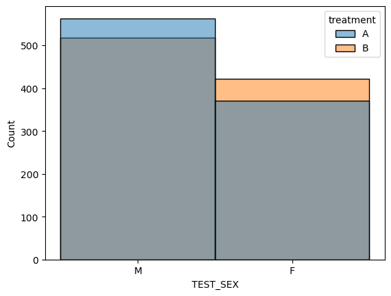
임의화로 지정한 두 그룹에 대하여 나이,몸무게,키에 대한 분포 비교

twogroup.groupby("treatment").describe()

	TEST_AGE								height					weight
	count	mean	std	min	25%	50%	75%	max	count	mean	...	75%	max	count	mean	std	min	25%	50%	75%	max
treatment
A	934.0	35.616702	17.432484	11.0	21.0	29.0	50.75	84.0	934.0	167.455353	...	174.5	195.2	934.0	67.466381	13.359358	34.1	57.925	66.85	75.300	132.3
B	940.0	35.329787	16.892562	11.0	22.0	28.5	48.00	83.0	940.0	166.716064	...	173.0	190.6	940.0	66.154362	12.926716	31.1	56.400	64.65	75.025	122.6

2 rows × 24 columns

sns.histplot(data=twogroup,x="TEST_AGE",hue="treatment")

<AxesSubplot:xlabel='TEST_AGE', ylabel='Count'>

sns.histplot(data=twogroup,x="weight",hue="treatment")

<AxesSubplot:xlabel='weight', ylabel='Count'>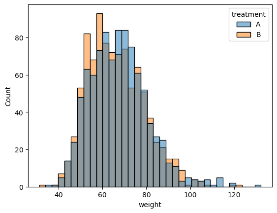

sns.histplot(data=twogroup,x="TEST_AGE",hue="treatment")

<AxesSubplot:xlabel='TEST_AGE', ylabel='Count'>

sns.histplot(data=twogroup,x="TEST_SEX",hue="treatment")

<AxesSubplot:xlabel='TEST_SEX', ylabel='Count'>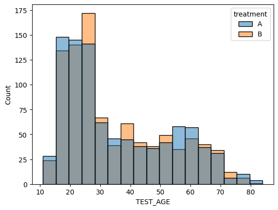

결과

처리를 제외한 다른 요인들의 분포가 각각의 그룹에서 유사하게 나타냄
처리를 제외한 다른 요인들로 인한 효과의 차이가 나타날 가능성 거의 없음.
“실험에서 처리를 임의화를 통하여 배정하면 두 그룹을 공정하게 비교할 수 있음”을 확인!

A/B test

두 그룹간의 차이가 있는지 비교.
유의성 검정을 통해 수행할 수 있음.

filename = "https://ilovedata.github.io/teaching/bigdata2/data/drug.csv"
three_drug_wide = pd.read_csv(filename)
three_drug_wide.head(10)

	Placebo	Old	New
0	31	23	23
1	28	17	17
2	34	29	11
3	36	23	11
4	33	17	9
5	27	17	16
6	39	22	16
7	25	17	14
8	23	23	17
9	29	25	18

three_drug_wide.describe()

	Placebo	Old	New
count	20.000000	20.000000	20.000000
mean	31.550000	20.900000	14.850000
std	4.334379	5.990343	4.319783
min	23.000000	5.000000	7.000000
25%	28.750000	17.000000	11.000000
50%	31.500000	21.000000	15.000000
75%	34.500000	24.250000	17.000000
max	39.000000	33.000000	24.000000

three_drug_wide.info()

<class 'pandas.core.frame.DataFrame'>
RangeIndex: 20 entries, 0 to 19
Data columns (total 3 columns):
 #   Column   Non-Null Count  Dtype
---  ------   --------------  -----
 0   Placebo  20 non-null     int64
 1   Old      20 non-null     int64
 2   New      20 non-null     int64
dtypes: int64(3)
memory usage: 608.0 bytes

pd.melt(frame,id_vars,value_vars,var_name,value_name)
- frame : long형으로 바꿀 df
- value_vars : value가 될 variable. 즉 값으로 바꿀 열들
- var_name : “variable” column이 이름. variable컬럼에는 column이름들이 포함되어 있음
- value_name : “value” column의 이름. value column에는 값들이 들어 있음.

three_drug_long = pd.melt(frame = three_drug_wide,value_vars = ["Placebo","Old","New"],var_name = "treatment",value_name = "Value")
three_drug_long.sample(10)

	treatment	Value
41	New	17
18	Placebo	30
46	New	16
17	Placebo	32
11	Placebo	36
55	New	17
48	New	17
51	New	7
0	Placebo	31
16	Placebo	30

cond = three_drug_long[three_drug_long.treatment == "Old"].index
two_drug = three_drug_long.drop(index=cond_col).reset_index(drop=True)
two_drug.head(10)

	treatment	Value
0	Placebo	31
1	Placebo	28
2	Placebo	34
3	Placebo	36
4	Placebo	33
5	Placebo	27
6	Placebo	39
7	Placebo	25
8	Placebo	23
9	Placebo	29

two_drug.groupby("treatment").describe()

	Value
	count	mean	std	min	25%	50%	75%	max
treatment
New	20.0	14.85	4.319783	7.0	11.00	15.0	17.0	24.0
Placebo	20.0	31.55	4.334379	23.0	28.75	31.5	34.5	39.0

temp = two_drug.groupby("treatment").mean().reset_index() #인덱스 있으면 불편,바로 reset!
temp

	treatment	Value
0	New	14.85
1	Placebo	31.55

x_p = float(temp[temp.treatment == "Placebo"].Value)
x_n = float(temp[temp.treatment == "New"].Value)
test_stat =  x_p - x_n
test_stat

16.700000000000003

two_drug.sample(5)

	treatment	Value
14	Placebo	33
10	Placebo	36
8	Placebo	23
34	New	18
29	New	18

def diff_mean(df,group_label,treatments = None):
    """
    df를 받아서 검정통계량을 계산해주는 함수. 검정통계량은 두 그룹간의 평균의 차이
        df : dataframe
        group_label : 처리가 적용된 변수명(그룹화 레이블)
        treatments : 비교하고 싶은 두 개의 처리명
    return : A 그룹 평균 - B 그룹 평균
    """
    df_group = df.groupby(group_label)
    temp = df_group.mean().reset_index()
    test_stat = float(temp[temp[group_label] == treatments[0]].Value) - float(temp[temp[group_label] == treatments[1]].Value)
    return test_stat

diff_mean(three_drug_long,"treatment",treatments = ["Placebo","New"])

16.700000000000003

two_drug_permuted

	treatment	Value	permuted_treatment
0	Placebo	31	New
1	Placebo	28	New
2	Placebo	34	Placebo
3	Placebo	36	Placebo
4	Placebo	33	Placebo
5	Placebo	27	Placebo
6	Placebo	39	New
7	Placebo	25	New
8	Placebo	23	Placebo
9	Placebo	29	New
10	Placebo	36	Placebo
11	Placebo	36	Placebo
12	Placebo	32	New
13	Placebo	30	New
14	Placebo	33	Placebo
15	Placebo	39	Placebo
16	Placebo	30	New
17	Placebo	32	Placebo
18	Placebo	30	New
19	Placebo	28	New
20	New	23	Placebo
21	New	17	New
22	New	11	New
23	New	11	New
24	New	9	New
25	New	16	New
26	New	16	Placebo
27	New	14	Placebo
28	New	17	Placebo
29	New	18	Placebo
30	New	10	New
31	New	7	Placebo
32	New	14	New
33	New	24	New
34	New	18	Placebo
35	New	17	Placebo
36	New	14	New
37	New	14	Placebo
38	New	16	Placebo
39	New	11	New

treatment = two_drug.treatment
two_drug_permuted = two_drug

random_permuted_treatment = treatment.sample(frac=1.0,replace=False).reset_index(drop=True) 
#reset_index안하면 sample로 shuffle을 해도 안섞임! 아마 인덱스끼리 매칭해주는 기능 있는 듯.
random_permuted_treatment.head(10)

0        New
1        New
2    Placebo
3        New
4    Placebo
5        New
6    Placebo
7        New
8        New
9        New
Name: treatment, dtype: object

two_drug_permuted = two_drug
two_drug_permuted["permuted_treatment"] = random_permuted_treatment
two_drug_permuted

	treatment	Value	permuted_treatment
0	Placebo	31	New
1	Placebo	28	New
2	Placebo	34	Placebo
3	Placebo	36	New
4	Placebo	33	Placebo
5	Placebo	27	New
6	Placebo	39	Placebo
7	Placebo	25	New
8	Placebo	23	New
9	Placebo	29	New
10	Placebo	36	Placebo
11	Placebo	36	New
12	Placebo	32	Placebo
13	Placebo	30	Placebo
14	Placebo	33	New
15	Placebo	39	Placebo
16	Placebo	30	Placebo
17	Placebo	32	New
18	Placebo	30	Placebo
19	Placebo	28	Placebo
20	New	23	Placebo
21	New	17	Placebo
22	New	11	New
23	New	11	New
24	New	9	New
25	New	16	New
26	New	16	New
27	New	14	Placebo
28	New	17	New
29	New	18	Placebo
30	New	10	Placebo
31	New	7	New
32	New	14	New
33	New	24	Placebo
34	New	18	Placebo
35	New	17	New
36	New	14	Placebo
37	New	14	New
38	New	16	Placebo
39	New	11	Placebo

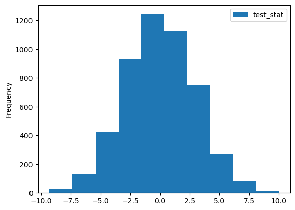
diff_mean(two_drug_permuted,"permuted_treatment",["Placebo","New"])

3.1999999999999993

B = 5000

test_stat_permuted = pd.DataFrame({"test_stat":np.zeros(B)})
treatment = two_drug.treatment

for i in np.arange(B):
    random_permuted_treatment = treatment.sample(frac=1.0,replace=False).reset_index(drop=True)
    two_drug_permuted = two_drug
    two_drug_permuted["permuted_treatment"] = random_permuted_treatment
    test_stat_permuted.loc[i,"test_stat"] = diff_mean(two_drug_permuted,"permuted_treatment",["Placebo","New"])

test_stat_permuted.plot.hist()

<AxesSubplot:ylabel='Frequency'>

p_value = np.mean(test_stat_permuted.test_stat > test_stat)
p_value

0.0